Tabular data modeling - with Tensorflow

tabular

tensorflow

In this notebook I try to use a competition dataset of log parameters of a server and classify if there was an attempt to attack the server

Published

June 24, 2020

“Tabular data modeling - with Tensorflow”

“In this notebook I try to use a competition dataset of log parameters of a server and classify if there was an attempt to attack the server”

In this notebook, I was giving a shot with Tensorflow for tabular data modeling, this particular competition data is quite imbalanced as you will see in this notebook a little later, This example is more or else fully adapted from the example from Tensorflow docs

Import required libraries

For Modeling

Show code

import tensorflow as tf
from tensorflow import keras

For Getting data from file to variable

Show code

import numpy as np
import pandas as pd

For Visualization

Show code

import seaborn as sns
import matplotlib as mpl
import matplotlib.pyplot as plt

/usr/local/lib/python3.6/dist-packages/statsmodels/tools/_testing.py:19: FutureWarning: pandas.util.testing is deprecated. Use the functions in the public API at pandas.testing instead.
  import pandas.util.testing as tm

For Evaluation and preprocessing

Show code

import sklearn
from sklearn.metrics import confusion_matrix
from sklearn.model_selection import train_test_split
from sklearn.preprocessing import StandardScaler
from sklearn.impute import SimpleImputer

Download data

Show code

#hide
import requests

#This link may not work
zip_file = requests.get('https://he-s3.s3.amazonaws.com/media/hackathon/novartis-data-science-hiring-challenge/predict-if-the-server-will-be-hacked-a1889487/6a62a5b4967411ea.zip?Signature=MXSW61lba65toXKZb6GJMMwKohs%3D&Expires=1592455446&AWSAccessKeyId=AKIA6I2ISGOYH7WWS3G5')

with open('data.zip', 'wb') as f:
    f.write(zip_file.content)

Show code

!unzip data.zip

Archive:  data.zip
   creating: Dataset/
  inflating: Dataset/Train.csv       
  inflating: Dataset/sample_submission.csv  
  inflating: Dataset/Test.csv

Show code

import pandas as pd
from pathlib import Path

DATA_PATH = Path('/content/Dataset')

train_data = pd.read_csv(DATA_PATH/'Train.csv', index_col=0, infer_datetime_format=True, converters={'DATE':pd.to_datetime})
train_data.head()

	DATE	X_1	X_2	X_3	X_4	X_5	X_6	X_7	X_8	X_9	X_10	X_11	X_12	X_13	X_14	X_15	MULTIPLE_OFFENSE
INCIDENT_ID
CR_102659	2004-07-04	0	36	34	2	1	5	6	1	6	1	174	1.0	92	29	36	0
CR_189752	2017-07-18	1	37	37	0	0	11	17	1	6	1	236	1.0	103	142	34	1
CR_184637	2017-03-15	0	3	2	3	5	1	0	2	3	1	174	1.0	110	93	34	1
CR_139071	2009-02-13	0	33	32	2	1	7	1	1	6	1	249	1.0	72	29	34	1
CR_109335	2005-04-13	0	33	32	2	1	8	3	0	5	1	174	0.0	112	29	43	1

Target Distribution

Show code

train_data['MULTIPLE_OFFENSE'].value_counts().plot.bar()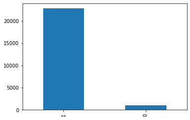

Show code

neg, pos = np.bincount(train_data['MULTIPLE_OFFENSE'])
total = neg + pos
print('Examples:\n    Total: {}\n    Positive: {} ({:.2f}% of total)\n'.format(
    total, pos, 100 * pos / total))

Examples:
    Total: 23856
    Positive: 22788 (95.52% of total)

We do have an imbalanced dataset, as shown above, 95% of the targets are positive (Class 1).

Data Preprocessing

Show code

seed=98
np.random.seed(seed=seed)
tf.random.set_seed(seed)

We shall drop the date column and try to model with only the logging parameters

Show code

cleaned_df = train_data.drop('DATE', axis='columns')

We split the training data to three train, test and eval sets

Show code

# Use a utility from sklearn to split and shuffle our dataset.
train_df, test_df = train_test_split(cleaned_df, test_size=0.2,
                                     random_state=seed, stratify=cleaned_df['MULTIPLE_OFFENSE'])

Show code

train_df, val_df = train_test_split(train_df, test_size=0.2,
                                    random_state=seed, stratify=train_df['MULTIPLE_OFFENSE'])

Show code

# Form np arrays of labels and features.
train_labels = np.array(train_df.pop('MULTIPLE_OFFENSE'))
bool_train_labels = train_labels != 0
val_labels = np.array(val_df.pop('MULTIPLE_OFFENSE'))
test_labels = np.array(test_df.pop('MULTIPLE_OFFENSE'))

train_features = np.array(train_df)
val_features = np.array(val_df)
test_features = np.array(test_df)

Create a preprocessing pipeline with scikit-learn

Show code

from sklearn.pipeline import Pipeline

preproc_pipe = Pipeline([
                 ('median_imputer', SimpleImputer(strategy='median')),
                 ('scaler', StandardScaler())
])

Show code

train_features = preproc_pipe.fit_transform(train_features)

val_features = preproc_pipe.transform(val_features)
test_features = preproc_pipe.transform(test_features)

# ensure that the values are within a range
train_features = np.clip(train_features, -5, 5)
val_features = np.clip(val_features, -5, 5)
test_features = np.clip(test_features, -5, 5)

Check the dimensions of our data

Show code

print('Training labels shape:', train_labels.shape)
print('Validation labels shape:', val_labels.shape)
print('Test labels shape:', test_labels.shape)

print('Training features shape:', train_features.shape)
print('Validation features shape:', val_features.shape)
print('Test features shape:', test_features.shape)

Training labels shape: (15267,)
Validation labels shape: (3817,)
Test labels shape: (4772,)
Training features shape: (15267, 15)
Validation features shape: (3817, 15)
Test features shape: (4772, 15)

Let’s check if our preprocessing has shown a distinction between the classes of the dataset

Show code

pos_df = pd.DataFrame(train_features[ bool_train_labels], columns = train_df.columns)
neg_df = pd.DataFrame(train_features[~bool_train_labels], columns = train_df.columns)

sns.jointplot(pos_df['X_10'], pos_df['X_15'],
              kind='hex', xlim = (-1,1), ylim = (-1,1))
plt.suptitle("Positive distribution")

sns.jointplot(neg_df['X_10'], neg_df['X_15'],
              kind='hex', xlim = (-1,1), ylim = (-1,1))
_ = plt.suptitle("Negative distribution")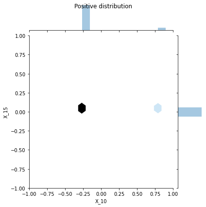

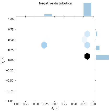
There is a slight difference in terms of the value, (ie) for the positive class the distribution is slightly on the negative side of zero, and the negative class is slightly on the positive side of zero

Model setup

Let’s setup the model layers and the evaluation metrics

Show code

# Function to plot losses
def plot_loss(history, label, n):
    # Use a log scale to show the wide range of values.
    plt.semilogy(history.epoch,  history.history['loss'],
                color=colors[n], label='Train '+label)
    plt.semilogy(history.epoch,  history.history['val_loss'],
            color=colors[n], label='Val '+label,
            linestyle="--")
    plt.xlabel('Epoch')
    plt.ylabel('Loss')

    plt.legend()

Show code

METRICS = [
      keras.metrics.TruePositives(name='tp'),
      keras.metrics.FalsePositives(name='fp'),
      keras.metrics.TrueNegatives(name='tn'),
      keras.metrics.FalseNegatives(name='fn'), 
      keras.metrics.BinaryAccuracy(name='accuracy'),
      keras.metrics.Precision(name='precision'),
      keras.metrics.Recall(name='recall'),
      keras.metrics.AUC(name='auc'),
]

def make_model(metrics=METRICS, output_bias=None):
    if output_bias is not None:
        output_bias = tf.keras.initializers.Constant(output_bias)

    model = keras.Sequential([
        keras.layers.Dense(
            16, activation='relu',
            input_shape=(train_features.shape[-1],)),
        keras.layers.Dropout(0.5),
        keras.layers.Dense(1, activation='sigmoid',
                            bias_initializer=output_bias),
    ])
    model.compile(optimizer=keras.optimizers.Adam(lr=1e-3),
                  loss=keras.losses.BinaryCrossentropy(),
                  metrics=metrics)
    return model

Set constants and callbacks

Show code

EPOCHS = 500
BATCH_SIZE = 4096

early_stopping = tf.keras.callbacks.EarlyStopping(
    monitor='val_recall', 
    verbose=1,
    patience=10,
    mode='max',
    restore_best_weights=True)

Calculate initial bias for a smooth training

Show code

initial_bias = np.log([pos/neg])
initial_bias

array([3.06044634])

Show code

model = make_model(output_bias=initial_bias)

Show code

results = model.evaluate(train_features, train_labels, batch_size=BATCH_SIZE, verbose=0)
print("Loss: {:0.4f}".format(results[0]))

Loss: 0.2112

Show code

import os, tempfile
initial_weights = os.path.join(tempfile.mkdtemp(),'initial_weights')
model.save_weights(initial_weights)

Calculate class weights to set to the model

Show code

weight_for_0 = (1 / neg)*(total)/2.0 
weight_for_1 = (1 / pos)*(total)/2.0

class_weight = {0: weight_for_0, 1: weight_for_1}

print('Weight for class 0: {:.2f}'.format(weight_for_0))
print('Weight for class 1: {:.2f}'.format(weight_for_1))

Weight for class 0: 11.17
Weight for class 1: 0.52

Train the model

Show code

weighted_model = make_model()
weighted_model.load_weights(initial_weights)

weighted_history = weighted_model.fit(
    train_features,
    train_labels,
    batch_size=BATCH_SIZE,
    epochs=EPOCHS,
    callbacks = [early_stopping],
    validation_data=(val_features, val_labels),
    # The class weights go here
    class_weight=class_weight)

Epoch 1/500
4/4 [==============================] - 1s 260ms/step - loss: 2.1039 - tp: 32485.0000 - fp: 1406.0000 - tn: 131.0000 - fn: 329.0000 - accuracy: 0.9495 - precision: 0.9585 - recall: 0.9900 - auc: 0.4448 - val_loss: 0.2044 - val_tp: 3646.0000 - val_fp: 171.0000 - val_tn: 0.0000e+00 - val_fn: 0.0000e+00 - val_accuracy: 0.9552 - val_precision: 0.9552 - val_recall: 1.0000 - val_auc: 0.4527
Epoch 2/500
4/4 [==============================] - 0s 21ms/step - loss: 2.0170 - tp: 14580.0000 - fp: 683.0000 - tn: 0.0000e+00 - fn: 4.0000 - accuracy: 0.9550 - precision: 0.9553 - recall: 0.9997 - auc: 0.4581 - val_loss: 0.2020 - val_tp: 3646.0000 - val_fp: 171.0000 - val_tn: 0.0000e+00 - val_fn: 0.0000e+00 - val_accuracy: 0.9552 - val_precision: 0.9552 - val_recall: 1.0000 - val_auc: 0.4656
Epoch 3/500
4/4 [==============================] - 0s 20ms/step - loss: 1.9718 - tp: 14570.0000 - fp: 682.0000 - tn: 1.0000 - fn: 14.0000 - accuracy: 0.9544 - precision: 0.9553 - recall: 0.9990 - auc: 0.4609 - val_loss: 0.1997 - val_tp: 3646.0000 - val_fp: 171.0000 - val_tn: 0.0000e+00 - val_fn: 0.0000e+00 - val_accuracy: 0.9552 - val_precision: 0.9552 - val_recall: 1.0000 - val_auc: 0.4698
Epoch 4/500
4/4 [==============================] - 0s 21ms/step - loss: 1.9492 - tp: 14572.0000 - fp: 681.0000 - tn: 2.0000 - fn: 12.0000 - accuracy: 0.9546 - precision: 0.9554 - recall: 0.9992 - auc: 0.4661 - val_loss: 0.1975 - val_tp: 3646.0000 - val_fp: 171.0000 - val_tn: 0.0000e+00 - val_fn: 0.0000e+00 - val_accuracy: 0.9552 - val_precision: 0.9552 - val_recall: 1.0000 - val_auc: 0.4828
Epoch 5/500
4/4 [==============================] - 0s 22ms/step - loss: 1.9312 - tp: 14570.0000 - fp: 682.0000 - tn: 1.0000 - fn: 14.0000 - accuracy: 0.9544 - precision: 0.9553 - recall: 0.9990 - auc: 0.4605 - val_loss: 0.1955 - val_tp: 3646.0000 - val_fp: 171.0000 - val_tn: 0.0000e+00 - val_fn: 0.0000e+00 - val_accuracy: 0.9552 - val_precision: 0.9552 - val_recall: 1.0000 - val_auc: 0.4899
Epoch 6/500
4/4 [==============================] - 0s 21ms/step - loss: 1.8575 - tp: 14570.0000 - fp: 682.0000 - tn: 1.0000 - fn: 14.0000 - accuracy: 0.9544 - precision: 0.9553 - recall: 0.9990 - auc: 0.4825 - val_loss: 0.1936 - val_tp: 3646.0000 - val_fp: 171.0000 - val_tn: 0.0000e+00 - val_fn: 0.0000e+00 - val_accuracy: 0.9552 - val_precision: 0.9552 - val_recall: 1.0000 - val_auc: 0.4988
Epoch 7/500
4/4 [==============================] - 0s 20ms/step - loss: 1.8257 - tp: 14560.0000 - fp: 679.0000 - tn: 4.0000 - fn: 24.0000 - accuracy: 0.9540 - precision: 0.9554 - recall: 0.9984 - auc: 0.4858 - val_loss: 0.1918 - val_tp: 3646.0000 - val_fp: 171.0000 - val_tn: 0.0000e+00 - val_fn: 0.0000e+00 - val_accuracy: 0.9552 - val_precision: 0.9552 - val_recall: 1.0000 - val_auc: 0.5161
Epoch 8/500
4/4 [==============================] - 0s 20ms/step - loss: 1.7717 - tp: 14555.0000 - fp: 677.0000 - tn: 6.0000 - fn: 29.0000 - accuracy: 0.9538 - precision: 0.9556 - recall: 0.9980 - auc: 0.5054 - val_loss: 0.1902 - val_tp: 3646.0000 - val_fp: 171.0000 - val_tn: 0.0000e+00 - val_fn: 0.0000e+00 - val_accuracy: 0.9552 - val_precision: 0.9552 - val_recall: 1.0000 - val_auc: 0.5260
Epoch 9/500
4/4 [==============================] - 0s 22ms/step - loss: 1.7657 - tp: 14551.0000 - fp: 678.0000 - tn: 5.0000 - fn: 33.0000 - accuracy: 0.9534 - precision: 0.9555 - recall: 0.9977 - auc: 0.5002 - val_loss: 0.1886 - val_tp: 3646.0000 - val_fp: 171.0000 - val_tn: 0.0000e+00 - val_fn: 0.0000e+00 - val_accuracy: 0.9552 - val_precision: 0.9552 - val_recall: 1.0000 - val_auc: 0.5330
Epoch 10/500
4/4 [==============================] - 0s 25ms/step - loss: 1.7285 - tp: 14539.0000 - fp: 678.0000 - tn: 5.0000 - fn: 45.0000 - accuracy: 0.9526 - precision: 0.9554 - recall: 0.9969 - auc: 0.5037 - val_loss: 0.1872 - val_tp: 3646.0000 - val_fp: 171.0000 - val_tn: 0.0000e+00 - val_fn: 0.0000e+00 - val_accuracy: 0.9552 - val_precision: 0.9552 - val_recall: 1.0000 - val_auc: 0.5431
Epoch 11/500
1/4 [======>.......................] - ETA: 0s - loss: 1.5431 - tp: 3918.0000 - fp: 166.0000 - tn: 1.0000 - fn: 11.0000 - accuracy: 0.9568 - precision: 0.9594 - recall: 0.9972 - auc: 0.5130Restoring model weights from the end of the best epoch.
4/4 [==============================] - 0s 22ms/step - loss: 1.6912 - tp: 14541.0000 - fp: 675.0000 - tn: 8.0000 - fn: 43.0000 - accuracy: 0.9530 - precision: 0.9556 - recall: 0.9971 - auc: 0.5073 - val_loss: 0.1860 - val_tp: 3646.0000 - val_fp: 171.0000 - val_tn: 0.0000e+00 - val_fn: 0.0000e+00 - val_accuracy: 0.9552 - val_precision: 0.9552 - val_recall: 1.0000 - val_auc: 0.5554
Epoch 00011: early stopping

We have got a good validation recall of 0.9026

Show code

mpl.rcParams['figure.figsize'] = (12, 10)
colors = plt.rcParams['axes.prop_cycle'].by_key()['color']

Show code

plot_loss(weighted_history, "Weighted", n=0)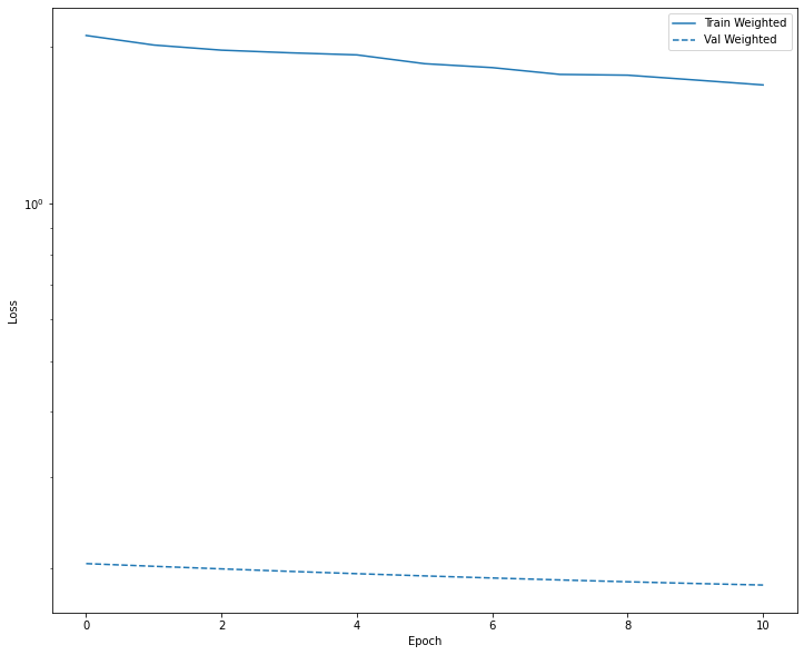

Looks like there still could be some room for improvement

Show code

def plot_metrics(history):
    metrics =  ['loss', 'auc', 'precision', 'recall']
    for n, metric in enumerate(metrics):
        name = metric.replace("_"," ").capitalize()
        plt.subplot(2,2,n+1)
        plt.plot(history.epoch,  history.history[metric], color=colors[0], label='Train')
        plt.plot(history.epoch, history.history['val_'+metric],
                    color=colors[0], linestyle="--", label='Val')
        plt.xlabel('Epoch')
        plt.ylabel(name)
        if metric == 'loss':
            plt.ylim([0, plt.ylim()[1]])
        elif metric == 'auc':
            plt.ylim([0.8,1])
        else:
            plt.ylim([0,1])

        plt.legend()

Show code

plot_metrics(weighted_history)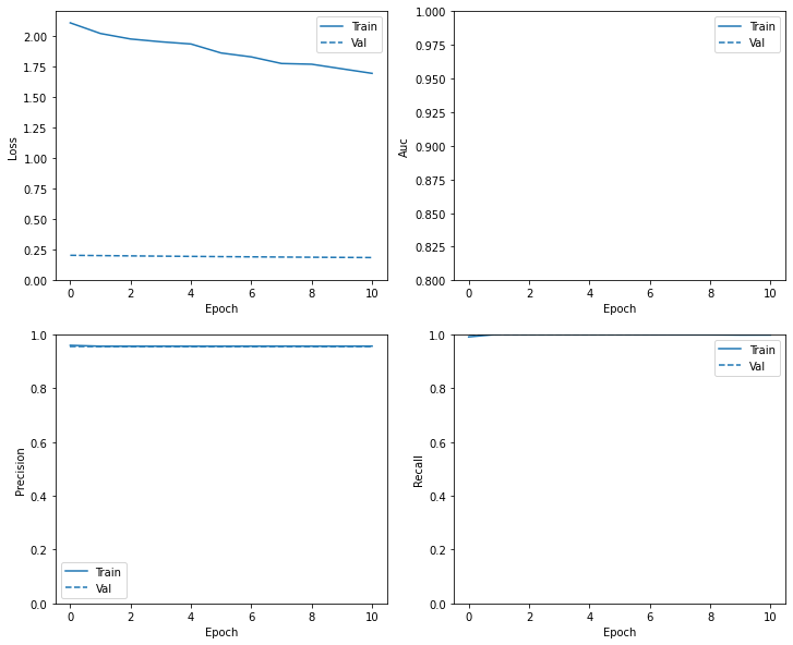

Predict with test data

Show code

test_data = pd.read_csv(DATA_PATH/'Test.csv', index_col=0)
test_data.drop('DATE', axis='columns', inplace=True)

Show code

proc_test = preproc_pipe.transform(np.array(test_data))

Show code

preds = np.argmax(weighted_model.predict(proc_test), axis=-1)

Show code

sub_df = pd.DataFrame(
    {'INCIDENT_ID':test_data.index,
     'MULTIPLE_OFFENSE':preds},
     )
sub_df.head()

	INCIDENT_ID	MULTIPLE_OFFENSE
0	CR_195453	0
1	CR_103520	0
2	CR_196089	0
3	CR_112195	0
4	CR_149832	0

Show code

sub_df.to_csv('submission_df.csv', index=False)

Show code

sub_df['MULTIPLE_OFFENSE'].value_counts()

0    15903
Name: MULTIPLE_OFFENSE, dtype: int64

I tried with various batch sizes and epochs to try to get it predict the classes differently maybe I should also try to change the model structure to achieve a different result because this submission only scored 50 recall on the competition test set.

I will also post other notebooks very soon, which will use machine learning based decision tree and random forest methods which performed way better on this problem.