Recommending a product price for a seller

This is another take home assignment that I did for a company as part of their interview process

“Recommending a product price for a seller”

“This is another take home assignment that I did for a company as part of their interview process”

This blog post has the code and details, of the take home project that I did for a company as part of their interview process, they gave me a dataset with sales details of a clothes/accessories from their website, the task was to make a price prediction/suggestion for a piece of wardrobe that the customer would like to sell on their company’s platform.

Prepare data and libraries

!unzip /content/ds-take-home-dataset.zip

Archive:  /content/ds-take-home-dataset.zip
  inflating: ds-take-home-dataset.csv  

!pip install -U scikit-learn

Collecting scikit-learn
  Downloading https://files.pythonhosted.org/packages/5c/a1/273def87037a7fb010512bbc5901c31cfddfca8080bc63b42b26e3cc55b3/scikit_learn-0.23.2-cp36-cp36m-manylinux1_x86_64.whl (6.8MB)
     |████████████████████████████████| 6.8MB 5.3MB/s 
Collecting threadpoolctl>=2.0.0
  Downloading https://files.pythonhosted.org/packages/f7/12/ec3f2e203afa394a149911729357aa48affc59c20e2c1c8297a60f33f133/threadpoolctl-2.1.0-py3-none-any.whl
Requirement already satisfied, skipping upgrade: scipy>=0.19.1 in /usr/local/lib/python3.6/dist-packages (from scikit-learn) (1.4.1)
Requirement already satisfied, skipping upgrade: numpy>=1.13.3 in /usr/local/lib/python3.6/dist-packages (from scikit-learn) (1.18.5)
Requirement already satisfied, skipping upgrade: joblib>=0.11 in /usr/local/lib/python3.6/dist-packages (from scikit-learn) (0.16.0)
Installing collected packages: threadpoolctl, scikit-learn
  Found existing installation: scikit-learn 0.22.2.post1
    Uninstalling scikit-learn-0.22.2.post1:
      Successfully uninstalled scikit-learn-0.22.2.post1
Successfully installed scikit-learn-0.23.2 threadpoolctl-2.1.0

Import Required Libraries

#collapse
import json
import pandas as pd
import numpy as np

from sklearn.model_selection import train_test_split
from sklearn.preprocessing import RobustScaler

import matplotlib.pyplot as plt

from joblib import dump
import os
import json

#collapse
file_path = r'/content/drive/My Drive/poshmark_files'

#collapse
np.random.seed(0)

Explore the dataset

#hide_input
data = pd.read_csv('/content/ds-take-home-dataset.zip')
data.head()

	id	attr1	attr2	attr3	attr4	attr5	attr6	title	sold_price
0	742122	4	27	149.0	3808.0	1.0	99.0	one teaspoon bandit distressed denim shorts (23)	65.0
1	652751	4	3	89.0	1996.0	NaN	1500.0	gucci emily mini guccissima mini red leather bag	600.0
2	228229	4	26	301.0	5194.0	NaN	89.0	steve madden polka dot wedges 8.5 - wi06	12.0
3	645810	4	27	NaN	6335.0	NaN	0.0	crown & ivy navy blue floral print shorts	12.0
4	854374	4	22	302.0	3606.0	2.0	45.0	grey wide leg dress pants	22.0

#hide_input
data.info()

<class 'pandas.core.frame.DataFrame'>
RangeIndex: 1029850 entries, 0 to 1029849
Data columns (total 9 columns):
 #   Column      Non-Null Count    Dtype  
---  ------      --------------    -----  
 0   id          1029850 non-null  int64  
 1   attr1       1029850 non-null  int64  
 2   attr2       1029850 non-null  int64  
 3   attr3       843080 non-null   float64
 4   attr4       864417 non-null   float64
 5   attr5       495664 non-null   float64
 6   attr6       1029850 non-null  float64
 7   title       1029761 non-null  object 
 8   sold_price  1029850 non-null  float64
dtypes: float64(5), int64(3), object(1)
memory usage: 70.7+ MB

#hide_input
print('Rows: {0} and cols: {1}'.format(*data.shape))

Rows: 1029850 and cols: 9

#hide_input
print('Number of Listing Id labels: ', len(data.id.unique()))
print('Number of Listings in the Dataset: ', len(data))

Number of Listing Id labels:  999850
Number of Listings in the Dataset:  1029850

#hide_input
data.describe()

	id	attr1	attr2	attr3	attr4	attr5	attr6	sold_price
count	1.029850e+06	1.029850e+06	1.029850e+06	843080.000000	864417.000000	495664.000000	1.029850e+06	1.029850e+06
mean	4.999636e+05	3.792792e+00	1.611883e+01	170.677981	3026.511901	1.452339	4.572187e+09	1.959587e+02
std	2.886351e+05	5.353355e-01	1.087543e+01	91.907382	1842.932124	0.497728	4.594750e+12	1.440187e+03
min	1.000000e+00	1.000000e+00	1.000000e+00	1.000000	1.000000	1.000000	0.000000e+00	0.000000e+00
25%	2.500282e+05	4.000000e+00	3.000000e+00	89.000000	1453.000000	1.000000	2.700000e+01	1.500000e+01
50%	4.999745e+05	4.000000e+00	1.400000e+01	180.000000	2896.000000	1.000000	1.190000e+02	5.000000e+01
75%	7.499088e+05	4.000000e+00	2.600000e+01	252.000000	4425.000000	2.000000	6.000000e+02	2.790000e+02
max	9.998500e+05	4.000000e+00	3.500000e+01	306.000000	6640.000000	3.000000	4.662595e+15	8.979010e+05

There are missing values in some columns, so let’s start by analysing them first.

Target Distribution

#collapse
data[data['sold_price'] > 0].shape[0]

1009850

#collapse
data[data['sold_price'] == 0].shape[0]

20000

There are 20000 listings with no price details, we might be better off removing them

#hide
bdata['sold_price'].hist(bins=10)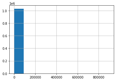

Missing value analysis

# make a list of the variables that contain missing values
vars_with_na = [var for var in data.columns if data[var].isnull().sum() > 0]

# get percentage of missing values
data[vars_with_na].isnull().mean()

attr3    0.181357
attr4    0.160638
attr5    0.518703
title    0.000086
dtype: float64

There is a sizeable chunk of missing data in feature attrs5 Let’s try to see whether they influence the price of a listing.

#collapse
def analyse_na_value(df, var):

    df = df.copy()

    # let's make a variable that indicates 1 if the observation was missing or zero otherwise
    df[var] = np.where(df[var].isnull(), 1, 0)

    # let's compare the median sold_price in the observations where data is missing
    # vs the observations where a value is available

    df.groupby(var)['sold_price'].median().plot.bar()

    plt.title(var)
    plt.show()


for var in vars_with_na:
    analyse_na_value(data, var)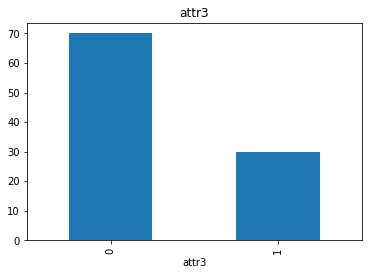

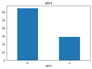
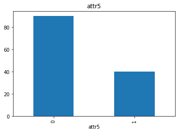
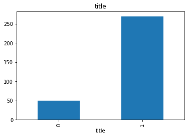
There is a change in the value of the sold_price when some attributes are empty, we should try to input this relationship when performing feature engineering

Almost all the features we have are categorical according to the instuctions given, let us try to analyze the only numeric variable attr6

Continous variable analysis

#collapse
data['attr6'].describe()

count    1.029850e+06
mean     4.572187e+09
std      4.594750e+12
min      0.000000e+00
25%      2.700000e+01
50%      1.190000e+02
75%      6.000000e+02
max      4.662595e+15
Name: attr6, dtype: float64

#collapse
var = 'attr6'
data[var].hist(bins=range(1, 10))
plt.ylabel('Number of listings')
plt.xlabel(var)
plt.title(var)
plt.show()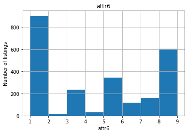

We can see that the variable is not normally distributed, We should remember to deal with this.

Unique value analysis

The feature attr6 is an interesting feature (Which can be clarified if it had a name) because the 20% values of that feature is Zero. This causes a confusion as to whether it is a categorical or numerical variable. A pie chart to view the counts.

#collapse
data['attr6'].value_counts().plot(kind='pie')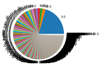

Percentage of zeros in attr6

#hide_input
data[data['attr6'] == 0].shape[0]/data.shape[0]

0.2049288731368646

Percentage of non-zeros in attr6

#hide_input
data[data['attr6'] > 0].shape[0]/data.shape[0]

0.7950711268631354

Categorical variable analysis

As per the instructions the categorical variables are

cat_vars ='attr1    attr2   attr3   attr4   attr5'.split('  ')

Let’s check the cardinality

#hide_input
data[cat_vars].nunique()

attr1       4
attr2      35
attr3     306
attr4    6640
attr5       3
dtype: int64

We do have huge number of categories in attr3 and attr4, let’s see about the rare labels with respect to the sold prices of the listing.

#collapse
def analyse_rare_labels(df, var, rare_perc):
    df = df.copy()

    # determine the % of observations per category
    tmp = df.groupby(var)['sold_price'].count() / len(df)

    # return categories that are rare
    return tmp[tmp < rare_perc]

# print categories that are present in less than
# .1 % of the observations

for var in cat_vars:
    print(analyse_rare_labels(data, var, 0.001))
    print()

Series([], Name: sold_price, dtype: float64)

attr2
4     0.000229
5     0.000979
7     0.000657
8     0.000653
10    0.000738
18    0.000559
23    0.000122
29    0.000257
34    0.000841
35    0.000574
Name: sold_price, dtype: float64

attr3
1.0      0.000804
2.0      0.000156
5.0      0.000304
6.0      0.000084
7.0      0.000766
           ...   
297.0    0.000006
299.0    0.000102
303.0    0.000664
305.0    0.000013
306.0    0.000770
Name: sold_price, Length: 197, dtype: float64

attr4
1.0       5.826091e-06
2.0       1.340001e-04
3.0       2.233335e-05
4.0       4.757974e-05
5.0       9.710152e-07
              ...     
6636.0    2.126523e-04
6637.0    2.524640e-05
6638.0    5.826091e-06
6639.0    9.710152e-07
6640.0    2.913046e-06
Name: sold_price, Length: 6510, dtype: float64

attr5
3.0    9.710152e-07
Name: sold_price, dtype: float64

attr4 has a lot of rare labels 6510 (98% of total unique labels)

We should try relating each category with the sold_price

#collapse
def analyse_discrete(df, var):
    df = df.copy()
    df.groupby(var)['sold_price'].median().plot.bar()
    plt.title(var)
    plt.ylabel('Median sold_price')
    plt.show()
    
for var in cat_vars:
    analyse_discrete(data, var)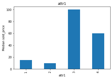

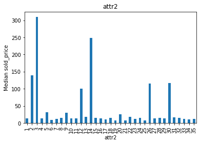
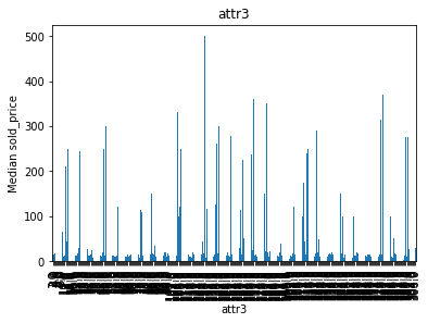
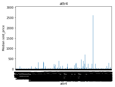
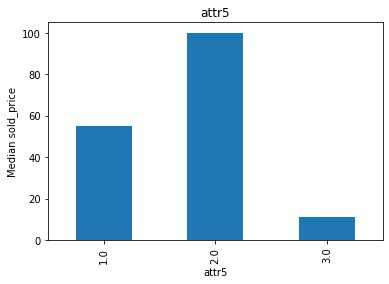
Outlier Analysis

#collapse
# let's make boxplots to visualise outliers in the continuous variables
def find_outliers(df, var):
    df = df.copy()

    df[var] = np.log1p(df[var])
    df.boxplot(column=var)
    plt.title(var)
    plt.ylabel(var)
    plt.show()


for var in ['attr6']:
    find_outliers(data, var)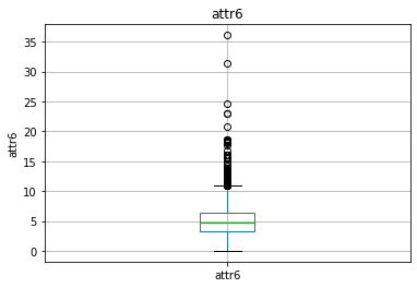

Feature Engineering

Import libraries for Feature engineering

from sklearn.pipeline import Pipeline
from sklearn.compose import ColumnTransformer
from sklearn.preprocessing import OneHotEncoder

Before we do the actual feature engineering, let’s split the data to train and test sets.

Since we need to be able to evaluate the model based on the bins of sold_price like 0-50, 50-100, 100-500, 500-1000 and 1000+., Let’s stratify the splitting by creating bins of the target variable

Avoid zero price listings

Train test split

zero_filter = data['sold_price'] > 0

bins = np.linspace(0, 1000, 10)

y_binned = np.digitize(data.loc[zero_filter, 'sold_price'], bins)

X_train, X_test, y_train, y_test = train_test_split(data[zero_filter].copy(),
                                                    data.loc[zero_filter, 'sold_price'].copy(),
                                                    test_size=0.3, stratify=y_binned)

bins

array([   0.        ,  111.11111111,  222.22222222,  333.33333333,
        444.44444444,  555.55555556,  666.66666667,  777.77777778,
        888.88888889, 1000.        ])

pd.Series(y_binned).value_counts()

1     570573
3     144418
2     104505
4      71537
5      44670
10     24617
6      19932
7      13618
8       9224
9       6756
dtype: int64

Missing values

Let’s check the percentage of missing values in the data

#collapse
# make a list of the variables that contain missing values
vars_with_na = [var for var in X_train.columns if data[var].isnull().sum() > 0]

# get percentage of missing values
X_train[vars_with_na].isnull().mean()

attr3    0.181816
attr4    0.160420
attr5    0.518667
title    0.000089
dtype: float64

#collapse
# make a list of the variables that contain missing values
vars_with_na = [var for var in X_test.columns if data[var].isnull().sum() > 0]

# get percentage of missing values
X_test[vars_with_na].isnull().mean()

attr3    0.180113
attr4    0.161057
attr5    0.518562
title    0.000083
dtype: float64

All the features with missing variables are categorical/string variables, so let’s just assign some arbitrary value missing to them.

# replace missing values with new label: "No Value Present" for title
# and with an arbitrary number for others

miss_cat = ['attr3', 'attr4', 'attr5']

X_train[miss_cat] = X_train[miss_cat].fillna(-9999)
X_test[miss_cat] = X_test[miss_cat].fillna(-9999)

X_train['title'] = X_train['title'].fillna('No Value Present')
X_test['title'] = X_test['title'].fillna('No Value Present')

#hide
# check that test set does not contain null values in the engineered variables

[var for var in vars_with_na if X_test[var].isnull().sum() > 0]

[]

#hide
# check that train set does not contain null values in the engineered variables

[var for var in vars_with_na if X_train[var].isnull().sum() > 0]

[]

As per the instruction the variable Id is kind of a temporal variable indicating the time in which the item was sold. So we can see if it helps with the prediction

Our only numeric variable as per the instruction is attr6 and it has no missing values so we do not need to touch that for now.

Handle infrequent/rare labels

#collapse
def find_frequent_labels(df, var, rare_perc):
    
    # function finds the labels that are shared by more than
    # a certain % of the listings in the dataset

    df = df.copy()

    tmp = df.groupby(var)['sold_price'].count() / len(df)

    return tmp[tmp > rare_perc].index


for var in cat_vars:
    
    # find the frequent categories
    frequent_ls = find_frequent_labels(X_train, var, 0.001)

    # replace rare categories by an arbitrary number
    X_train[var] = np.where(X_train[var].isin(
        frequent_ls), X_train[var], -999)
    
    X_test[var] = np.where(X_test[var].isin(
        frequent_ls), X_test[var], -999)

# this function will assign discrete values to the values of the variables,
# so that the smaller value corresponds to the category that shows the smaller
# mean sold_price

def replace_categories(train, test, var, target):

    # order the categories in a variable from that with the lowest
    # house sale price, to that with the highest
    ordered_labels = train.groupby([var])[target].mean().sort_values().index
    # create a dictionary of ordered categories to integer values
    ordinal_label = {k: i for i, k in enumerate(ordered_labels, 0)}
    with open(f'{var}.json', 'w') as f: json.dump(ordinal_label, f)

    # use the dictionary to replace the categorical strings by integers
    train[var] = train[var].map(ordinal_label)
    test[var] = test[var].map(ordinal_label)

cat_vars

['attr1', 'attr2', 'attr3', 'attr4', 'attr5']

for var in cat_vars:
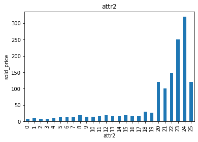
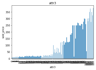
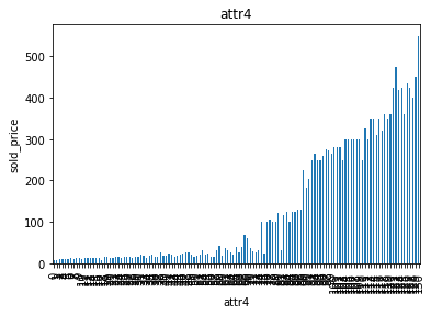
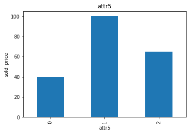
    replace_categories(X_train, X_test, var, 'sold_price')

# for displaying monotonic relationship
# between labels and target

def analyse_vars(df, var):
    # function plots median sold price per encoded category
    
    df = df.copy()
    df.groupby(var)['sold_price'].median().plot.bar()
    plt.title(var)
    plt.ylabel('sold_price')
    plt.show()
    
for var in cat_vars:
    analyse_vars(X_train, var)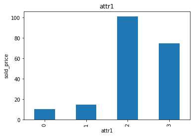

Feature scaling

num_vars = ['attr6', 'id']
numeric_transformer = Pipeline(steps=[
    ('scaler', RobustScaler())]
    )

Text Feature Extraction

from sklearn.feature_extraction.text import TfidfVectorizer
from sklearn.decomposition import TruncatedSVD

# using tfidf on the text data and reducing the vector dimensions with SVD
text_transformer = Pipeline(
    steps=[
           ('tfidf', TfidfVectorizer()),
           ('best', TruncatedSVD(n_components=5))
    ]
)
preprocessor = ColumnTransformer(
    transformers=[
        ('num', numeric_transformer, num_vars),
        ('text', text_transformer, 'title')
        ],
        remainder='passthrough'
)

Model Building

Let’s look at the target data in a scatter plot

#collapse
plt.scatter(x=range(len(y_train)), y=y_train)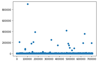

The target has outliers, So transforming the target might help the regression model to fit the data

Import required things for modeling

# to build the model
from sklearn.compose import TransformedTargetRegressor
from sklearn.svm import SVR
from sklearn.linear_model import Lasso, LassoLarsIC, RidgeCV, LinearRegression, RANSACRegressor, SGDRegressor
from sklearn.preprocessing import QuantileTransformer, quantile_transform

# to evaluate the model
from sklearn.metrics import mean_squared_error, r2_score, median_absolute_error
from math import sqrt

Target transformation with Quantiles

The snippet is more or less copied from scikit-learn’s example gallery, this graph shows the effect of transforming the target with quantiles.

# collapse
density_param = {'density':True}
y = X_train.loc[:, 'sold_price'].squeeze()
y_trans = quantile_transform(X_train.loc[:, 'sold_price'].values.reshape(-1, 1),
                             n_quantiles=300,
                             output_distribution='normal',
                             copy=True).squeeze()

f, (ax0, ax1) = plt.subplots(1, 2)

ax0.hist(y, bins=100, **density_param)
ax0.set_ylabel('Probability')
ax0.set_xlabel('Target')
ax0.set_title('Target distribution')

ax1.hist(y_trans, bins=100, **density_param)
ax1.set_ylabel('Probability')
ax1.set_xlabel('Target')
ax1.set_title('Transformed target distribution')

f.suptitle("Listing data: distance to price centers", y=0.035)
f.tight_layout(rect=[0.05, 0.05, 0.95, 0.95])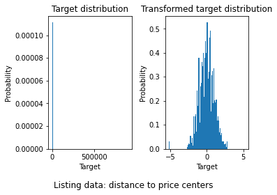

Put together the feature engineering pipeline and model

regr_trans = TransformedTargetRegressor(regressor=LassoLarsIC(normalize=False),
                                        transformer=QuantileTransformer(output_distribution='normal'))

model = Pipeline(steps=[('preprocessor', preprocessor),
                      ('regressor', regr_trans)],
                 memory='/content'
               )

Begin modeling

#hide
_ = X_train.pop('sold_price')
_ = X_test.pop('sold_price')

#hide
X_train.shape

(706895, 8)

Model using regularized linear regression

model.fit(X_train, y_train)

Model Structure

#hide
from sklearn import set_config
set_config(display='diagram')
model

Pipeline

Pipeline(memory='/content',
         steps=[('preprocessor',
                 ColumnTransformer(remainder='passthrough',
                                   transformers=[('num',
                                                  Pipeline(steps=[('scaler',
                                                                   RobustScaler())]),
                                                  ['attr6', 'id']),
                                                 ('text',
                                                  Pipeline(steps=[('tfidf',
                                                                   TfidfVectorizer()),
                                                                  ('best',
                                                                   TruncatedSVD(n_components=5))]),
                                                  'title')])),
                ('regressor',
                 TransformedTargetRegressor(regressor=SGDRegressor(max_iter=2000),
                                            transformer=QuantileTransformer(output_distribution='normal')))])

preprocessor: ColumnTransformer

ColumnTransformer(remainder='passthrough',
                  transformers=[('num',
                                 Pipeline(steps=[('scaler', RobustScaler())]),
                                 ['attr6', 'id']),
                                ('text',
                                 Pipeline(steps=[('tfidf', TfidfVectorizer()),
                                                 ('best',
                                                  TruncatedSVD(n_components=5))]),
                                 'title')])

num

['attr6', 'id']

RobustScaler

RobustScaler()

text

title

TfidfVectorizer

TfidfVectorizer()

TruncatedSVD

TruncatedSVD(n_components=5)

regressor: TransformedTargetRegressor

TransformedTargetRegressor(regressor=SGDRegressor(max_iter=2000),
                           transformer=QuantileTransformer(output_distribution='normal'))

SGDRegressor

SGDRegressor(max_iter=2000)

QuantileTransformer

QuantileTransformer(output_distribution='normal')

Try predicting on train and test data to evaluate fit

Evaluation

Let’s have a look at the mean square and median absolute errors of the train and test sets.

#collapse
# We will evaluate performance using the mean squared error and
# the root of the mean squared error and r2

# make predictions for train set
pred = model.predict(X_train)

# determine mse and rmse
print('train mse: {}'.format(int(
    mean_squared_error(y_train, pred))))
print('train rmse: {}'.format(int(
    sqrt(mean_squared_error(y_train, pred)))))
print('train r2: {}'.format(
    r2_score(y_train, pred)))
print()

# make predictions for test set
pred = model.predict(X_test)

# determine mse and rmse
print('test mse: {}'.format(int(
    mean_squared_error(y_test, pred))))
print('test rmse: {}'.format(int(
    sqrt(mean_squared_error(y_test, pred)))))
print('test r2: {}'.format(
    r2_score(y_test, pred)))
print()

print('Median listing price: ', int(y_train.median()))

train mse: 2384016
train rmse: 1544
train r2: 0.012738801579374459

test mse: 1420721
test rmse: 1191
test r2: -0.005001811084259344

Median listing price:  60

#collapse
# We will evaluate performance using the median abs error and
# the root of the mean squared error and r2

# make predictions for train set
pred = model.predict(X_train)

# determine mae
print('train mae: {}'.format(int(
    median_absolute_error(y_train, pred))))

print('train r2: {}'.format(
    r2_score(y_train, pred)))
print()

# make predictions for test set
pred = model.predict(X_test)

# determine mae
print('test mae: {}'.format(int(
    median_absolute_error(y_test, pred))))
print('test r2: {}'.format(
    r2_score(y_test, pred)))
print()

print('Median listing price: ', int(y_train.median()))

train mae: 37
train r2: 0.012738801579374459

test mae: 37
test r2: -0.005001811084259344

Median listing price:  60

It is kinda evident that the model has not performed well(looking at the \(r^2\) values) maybe I should have used another modeling method to get better results.

#hide
# let's evaluate our predictions respect to the sold price
plt.scatter(y_test, model.predict(X_test))
plt.xlabel('True Listing Price')
plt.ylabel('Predicted Listing Price')
plt.title('Evaluation of Lasso Predictions')

Text(0.5, 1.0, 'Evaluation of Lasso Predictions')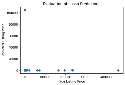

Let’s evaluate our predictions respect to the sold price, In the picture, The blue dots are predicted values and the red ones are the predicted values.

#collapse
plt.scatter(range(0, len(y_test)), y_test, color='red')
plt.scatter(range(0, len(X_test)), model.predict(X_test), color='blue')
plt.xlabel('record number')
plt.ylabel('Actual and Predicted Listing Price')
plt.title('Evaluation of Lasso Predictions')

Text(0.5, 1.0, 'Evaluation of Lasso Predictions')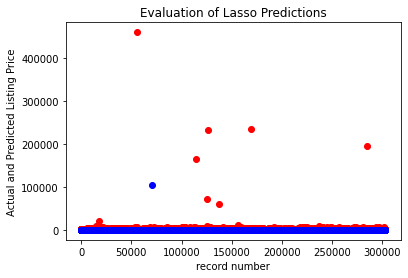

Error distribution

# let's evaluate the distribution of the errors: 

errors = y_test - model.predict(X_test)
errors.hist(bins=30)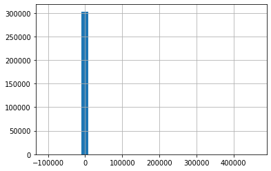

The chart is not very informative but the range of numbers in x axis gives an idea of the error range.

I also did another exercise for the same company, which deals with calculating the feature importances in a model agnostic way. You can have look at that here