Calculus - d2l.ai Exercises - Part 4

The fourth notebook in a series to be posted aiming to solve and understand exercises from d2l.ai curriculum on deep learning

“Calculus - d2l.ai Exercises - Part 4”

“The fourth notebook in a series to be posted aiming to solve and understand exercises from d2l.ai curriculum on deep learning”

Required Imports

#collapse
!pip install d2l

#collapse_show
%matplotlib inline
import numpy as np
from IPython import display
from d2l import tensorflow as d2l

Setup for plotting

#collapse
def use_svg_display():
    """Use the svg format to display a plot in Jupyter."""
    display.set_matplotlib_formats('svg')

def set_figsize(figsize=(3.5, 2.5)):
    """Set the figure size for matplotlib."""
    use_svg_display()
    d2l.plt.rcParams['figure.figsize'] = figsize

def set_axes(axes, xlabel, ylabel, xlim, ylim, xscale, yscale, legend):
    """Set the axes for matplotlib."""
    axes.set_xlabel(xlabel)
    axes.set_ylabel(ylabel)
    axes.set_xscale(xscale)
    axes.set_yscale(yscale)
    axes.set_xlim(xlim)
    axes.set_ylim(ylim)
    if legend:
        axes.legend(legend)
    axes.grid()

def plot(X, Y=None, xlabel=None, ylabel=None, legend=None, xlim=None,
         ylim=None, xscale='linear', yscale='linear',
         fmts=('-', 'm--', 'g-.', 'r:'), figsize=(3.5, 2.5), axes=None):
    """Plot data points."""
    if legend is None:
        legend = []

    set_figsize(figsize)
    axes = axes if axes else d2l.plt.gca()

    # Return True if `X` (tensor or list) has 1 axis
    def has_one_axis(X):
        return (hasattr(X, "ndim") and X.ndim == 1 or
                isinstance(X, list) and not hasattr(X[0], "__len__"))

    if has_one_axis(X):
        X = [X]
    if Y is None:
        X, Y = [[]] * len(X), X
    elif has_one_axis(Y):
        Y = [Y]
    if len(X) != len(Y):
        X = X * len(Y)
    axes.cla()
    for x, y, fmt in zip(X, Y, fmts):
        if len(x):
            axes.plot(x, y, fmt)
        else:
            axes.plot(y, fmt)
    set_axes(axes, xlabel, ylabel, xlim, ylim, xscale, yscale, legend)

Question 1: Plot the function \(y=f(x)=x^3−(1/x)\) and its tangent line when \(x=1\).

The derivative of \(f(x)\) here is \(f'(x) = 3x^2 + 1/x^2\) and by setting \(x=1\), we get 4, let’s try to simulate like they did.

def f(x):
    return x**3 - (x ** -1)

def numerical_lim(f, x, h):
    return (f(x + h) - f(x)) / h

h = 0.1
for i in range(10):
    print(f'h={h:.10f}, numerical limit={numerical_lim(f, 1, h):.10f}')
    h *= 0.1

Standard Output

h=0.1000000000, numerical limit=4.2190909091
h=0.0100000000, numerical limit=4.0201990099
h=0.0010000000, numerical limit=4.0020019990
h=0.0001000000, numerical limit=4.0002000200
h=0.0000100000, numerical limit=4.0000200002
h=0.0000010000, numerical limit=4.0000019997
h=0.0000001000, numerical limit=4.0000002022
h=0.0000000100, numerical limit=3.9999999868
h=0.0000000010, numerical limit=4.0000003310
h=0.0000000001, numerical limit=4.0000003310

We do see that the value approaches to 4. So \(y=4\) when \(x=1\), to find the equation of the tangent line to \(x^3−(1/x)\) at \(x=1\)

We already have the slope of the tangent line by substituting \(x=1\) on \(f'(x)\) which is \(4\), since a tangent line shares atleast one point with the original equation(\(f(x)\)), substituting the \(x\) in \(f(x)\) we get \(0\).

So the common(shared) point between \(f(x)\) and its tangent at \(x=1\) is \((1,0)\), we can use the slope \(4\) and the point \((1,0)\) to find the equation of the tangent line at \(x=1\) with the formula:

\[y - y_1 = m(x-x_1)\]

where the \(m\) is the slope and \(x_1\) and \(y_1\) are coordinates from the point which we found. Plugging in the values which we have into the equation we get the equation

\[ y = 4x - 4 \]

This is a good reference for another example of this method.

Let’s see if it is the tangent line by visualising it

x = np.arange(0.1, 3, 0.1)
plot(x, [f(x), 4 * x - 4], 'x', 'f(x)', legend=['f(x)', 'Tangent line (x=1)'])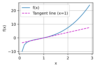

Question 2: Find the gradient of the function \(f(x) = 3x_1^2 + 5e^{x_2}\)

For gradient we need to calculate the partial derivatives of the function given with respect to its variables. (ie) \(\frac{\partial y}{\partial x_1}\) and \(\frac{\partial y}{\partial x_2}\)

\[\frac{\partial y}{\partial x_1} = 6x_1 \]

\[\frac{\partial y}{\partial x_2} = 5e^{x_2}\]

so the gradient will be \[\nabla_xf(x) = [6x_1, 5e^{x_2}]\]

Question 3: Find the gradient of \(f(x) = ∥x∥_2\).

For this function, it can be split into \(\sqrt{x^Tx}\).
Let’s consider \(u = x^Tx\) then our function would become $f(x) = $ or \(u^{1/2}\)

So now we have two variables \(u\) and \(x\), the gradient of the function would be

\[\frac{\partial y} {\partial u} . \frac{\partial y} {\partial x}\]
\[\frac{\partial y} {\partial u} = (1/2)*(u)^{-1/2} = \frac{1}{2 \sqrt u} = \frac{1}{2 ||x||_2}\]
\[\frac{\partial y} {\partial x} = \frac {\partial x^Tx} {\partial x} = 2x\]
\[\nabla_xf(x) = \frac{\partial y} {\partial u} . \frac{\partial y} {\partial x}\]

\[ = \frac{1}{2 ||x||_2} . 2x = \frac {x}{||x||_2}\]

Question 4: Can you write out the chain rule for the case where \(u=f(x,y,z)\) and \(x=x(a,b) , y=y(a,b)\) and $z=z(a,b) $?

We need to treat \(u\) as a function with variables \(x\), \(y\) and \(z\) and each of \(x,y,z\) as functions with variables \(a\) and \(b\)

so by applying chain rule we get

\[ \frac{\partial u}{\partial a} = \frac{\partial u}{\partial x}\frac{\partial x}{\partial a}+\frac{\partial u}{\partial y}\frac{\partial y}{\partial a}+\frac{\partial u}{\partial z}\frac{\partial z}{\partial a}\]
\[ \frac{\partial u}{\partial a} = \frac{\partial u}{\partial x}\frac{\partial x}{\partial b} + \frac{\partial u}{\partial y}\frac{\partial y}{\partial b}+\frac{\partial u}{\partial z}\frac{\partial z}{\partial b}\]